Is parking the bus worth it?
September 28, 2017
There has been an ongoing discussion on Twitter on whether it is better for underdogs to play defensively or offensively.
Werder Bremen is ill advised to focus on defense. In relegation race you need to focus on scoring. The old 4:3-Werder would do better.
— Goalimpact (@Goalimpact) September 27, 2017
Now, to me, it is a mathematical certainty that lower-scoring games are more random, and thus better for the underdog. Conversely, higher-scoring games are better for the favorites, who are more assured of winning as more goals lead to less random outcomes.
It is a pretty simple point, and it squares with the general perceptions people have about the football. Big teams play more defensive setups when playing against other big teams. Games against defensive-minded minnows like Burnley are feared more than those against attack-minded sides like Bournemouth. Most people who watch football intuitively feel like a team has got to defend when playing against a better team.
Most, but not all.
As every other claim made about football, this one also draws its fair share of resistance and pushback. People don’t always believe it, and they try to back their case up with data. Frequently, a lack of mathematical and statistical knowledge leads to mishandling of data, especially in football where we are dealing with small amounts of count data.
So I decided to show, using real data, how it is better for relegation contenders to be defensive and for title contenders to be attacking. I hope this empirical exercise will convince people that it really is an underlying mathematical feature we are dealing with here, even if they can’t fully understand the mathematics that go into it.
Our dataset contains 15 Premier League seasons, with points and goals.
## # A tibble: 300 x 5
##                 team  season points goals_for goals_against
##                <chr>   <chr>  <dbl>     <dbl>         <dbl>
##  1 Manchester United 2002/03     83        74            34
##  2           Arsenal 2002/03     78        85            42
##  3  Newcastle United 2002/03     69        63            48
##  4           Chelsea 2002/03     67        68            38
##  5         Liverpool 2002/03     64        61            41
##  6  Blackburn Rovers 2002/03     60        52            43
##  7           Everton 2002/03     59        48            49
##  8       Southampton 2002/03     52        43            46
##  9   Manchester City 2002/03     51        47            54
## 10 Tottenham Hotspur 2002/03     50        51            62
## # ... with 290 more rows
The goal is to model total points as a function of the goals scored and conceded. First we have to re-parameterize goals scored/conceded to an unconstrained scale, as we are going to use them in a linear model later. Count data such as goals is lower-bounded at zero, but there should be no limit to how bad a team’s attack is. We then calculate a measure of quality and a measure of attacking/defensive balance.
premier_league_historical_stats <-
  premier_league_historical_stats %>%
  mutate(

    # First, see how many goals the team scores relative to the average
    norm_attack = goals_for %>% divide_by(mean(goals_for)) %>%
      # Then, transform it into an unconstrained scale
      log(),
    # First, see how many goals the team concedes relative to the average
    norm_defense = goals_against %>% divide_by(mean(goals_against)) %>%
      # Invert it, so a higher defense is better
      raise_to_power(-1) %>%
      # Then, transform it into an unconstrained scale
      log(),

    # Now that we have normalized attack and defense ratings, we can compute
    # measures of quality and attacking balance

    quality = norm_attack + norm_defense,
    balance = norm_attack - norm_defense
  )
We now have two metrics, quality and balance, that capture how good and how attacking a team is, respectively. Incidentally, quality is exactly the log of the goal ratio, a metric that is familiar to football fans. balance is its lesser-kown sibling, that we can christen as goal product as it should map directly onto the product of the goals scored and the goals conceded.
These are the most attacking teams in the past 15 seasons:
## # A tibble: 300 x 6
##                    team  season points goals_for goals_against   balance
##                   <chr>   <chr>  <dbl>     <dbl>         <dbl>     <dbl>
##  1            Liverpool 2013/14     84       101            50 0.6808220
##  2            Blackpool 2010/11     39        55            78 0.5177205
##  3    Tottenham Hotspur 2007/08     46        66            61 0.4542071
##  4 West Bromwich Albion 2010/11     47        56            71 0.4417101
##  5      Manchester City 2013/14     86       102            37 0.3895692
##  6     Blackburn Rovers 2011/12     31        48            78 0.3815883
##  7    Manchester United 2012/13     89        86            43 0.3692259
##  8      AFC Bournemouth 2016/17     46        55            67 0.3657043
##  9              Arsenal 2011/12     70        74            49 0.3495639
## 10          Aston Villa 2007/08     60        71            51 0.3481840
## # ... with 290 more rows
And these are the most defensive:
## # A tibble: 300 x 6
##                 team  season points goals_for goals_against    balance
##                <chr>   <chr>  <dbl>     <dbl>         <dbl>      <dbl>
##  1           Chelsea 2004/05     95        72            15 -0.8616052
##  2   Manchester City 2006/07     42        29            44 -0.6948360
##  3            Fulham 2008/09     53        39            34 -0.6563993
##  4        Sunderland 2002/03     19        21            65 -0.6274118
##  5  Blackburn Rovers 2004/05     42        32            43 -0.6193855
##  6   Birmingham City 2005/06     34        28            50 -0.6020940
##  7         Liverpool 2005/06     82        57            25 -0.5843944
##  8     Middlesbrough 2016/17     28        27            53 -0.5801927
##  9           Burnley 2014/15     33        28            53 -0.5438251
## 10 Manchester United 2004/05     77        58            26 -0.5277820
## # ... with 290 more rows
Now we can fit a simple linear model of points, where the predictors are:
- Quality: the greater the quality, the higher the total points
- Interaction between quality and balance: according to our “hypothesis”, for high-quality teams, an attacking balance should lead to more points. For low-quality teams, the reverse should be true.
fit <-
  premier_league_historical_stats %>%
  lm(points ~ quality + quality:balance, data = .)

summary(fit)
##
## Call:
## lm(formula = points ~ quality + quality:balance, data = .)
##
## Residuals:
## Min 1Q Median 3Q Max
## -11.9838 -3.0554 -0.2553 2.8365 14.2059
##
## Coefficients:
## Estimate Std. Error t value Pr(>|t|)
## (Intercept) 52.2606 0.2510 208.19 < 2e-16 ***
## quality 32.9394 0.5473 60.18 < 2e-16 ***
## quality:balance 6.6145 1.6618 3.98 8.66e-05 ***
## ---
## Signif. codes: 0 '***' 0.001 '**' 0.01 '*' 0.05 '.' 0.1 ' ' 1
##
## Residual standard error: 4.347 on 297 degrees of freedom
## Multiple R-squared: 0.9343, Adjusted R-squared: 0.9338
## F-statistic: 2110 on 2 and 297 DF, p-value: < 2.2e-16I’ve shown the p-values above, in case you care about them (which you shouldn’t, but horses for courses, etc).
So we would expect a team of average quality and average balance to get about 52 points over a season. The team quality obviously has a huge impact on the team’s point return.
Most importantly, we see that the interaction term quality:balance is positive, meaning when both quality and balance are positive (i.e. attacking title contenders) a team will get more points and that when both are negative (i.e. defensive relegation battlers) it will also get more points.
This hopefully should prove our hypothesis. However, just to make sure, let’s look at it from a different angle. Let’s fit one model to attacking teams and another to defensive teams and see how they differ. We are expecting attacking teams’ points totals to display a stronger dependence on the team quality. In other words, defensive teams tend towards an average points return, whereas attacking teams tend towards an extreme (good or bad) points return.
Results in plot form:
premier_league_historical_stats %>%
  ggplot(aes(quality, points, fill = balance)) +
  geom_smooth(data = . %>% filter(balance > 0),
    method = "lm", color = scales::muted("red"), fill = scales::muted("red")
  ) +
  geom_smooth(data = . %>% filter(balance < 0),
    method = "lm", color = scales::muted("blue"), fill = scales::muted("blue")
  ) +
  geom_point(pch = 21) +
  scale_fill_gradient2(
    low = scales::muted("blue"),
    high = scales::muted("red"),
    midpoint = 0
  ) +
  theme_classic()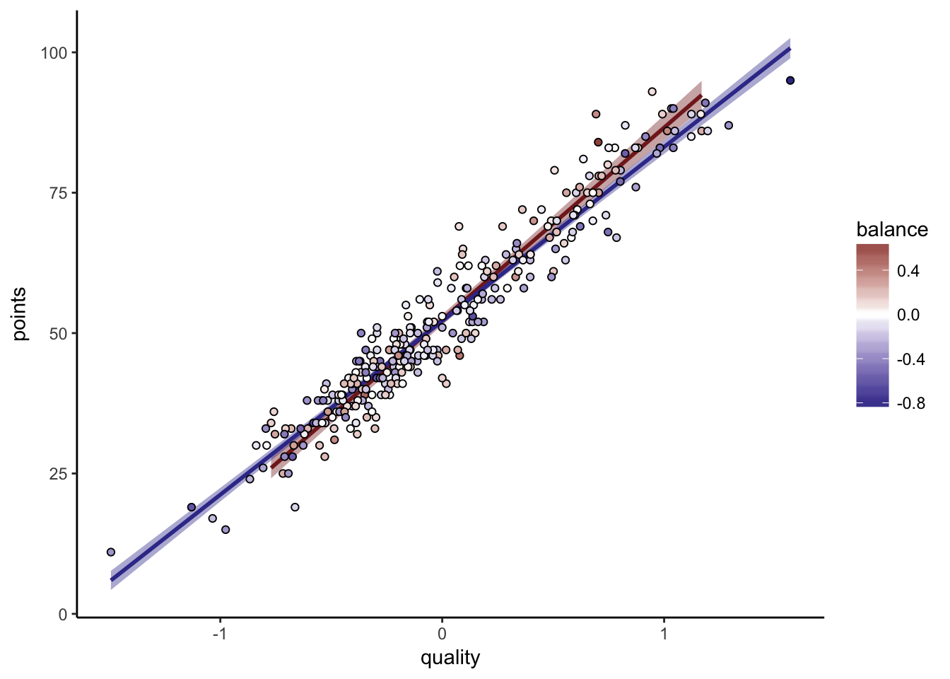
As we can see, the red line, fit on the attacking teams, has a greater slope than the blue line. The red dots are higher than the blue dots at high quality, but lower at low quality.
For good teams, it is better to be offensive, and for bad teams, it is better to be defensive
Bundesliga
Because I’m absolutely sure it will come up, I’ve gone through the same process for the Bundesliga:
##
## Call:
## lm(formula = points ~ quality + quality:balance, data = .)
##
## Residuals:
##     Min      1Q  Median      3Q     Max
## -9.8838 -2.4037 -0.2118  2.5132 12.8669
##
## Coefficients:
##                 Estimate Std. Error t value Pr(>|t|)
## (Intercept)      46.9071     0.2437 192.442  < 2e-16 ***
## quality          29.6913     0.6199  47.898  < 2e-16 ***
## quality:balance   8.7918     1.8896   4.653 5.16e-06 ***
## ---
## Signif. codes:  0 '***' 0.001 '**' 0.01 '*' 0.05 '.' 0.1 ' ' 1
##
## Residual standard error: 4.005 on 267 degrees of freedom
## Multiple R-squared:  0.9161, Adjusted R-squared:  0.9155
## F-statistic:  1457 on 2 and 267 DF,  p-value: < 2.2e-16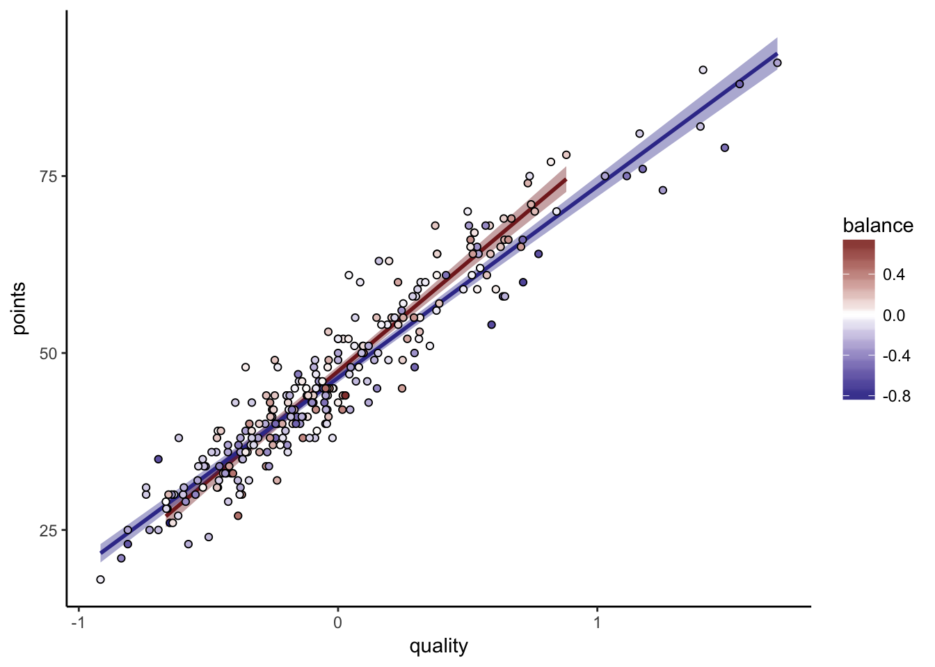
La Liga
I’ve also done La Liga for good measure:
##
## Call:
## lm(formula = points ~ quality + quality:balance, data = .)
##
## Residuals:
##      Min       1Q   Median       3Q      Max
## -11.7980  -2.8996  -0.2284   2.4030  11.9613
##
## Coefficients:
##                 Estimate Std. Error t value Pr(>|t|)
## (Intercept)      52.8459     0.2484 212.721  < 2e-16 ***
## quality          32.1389     0.5034  63.844  < 2e-16 ***
## quality:balance   6.6841     1.6117   4.147  4.4e-05 ***
## ---
## Signif. codes:  0 '***' 0.001 '**' 0.01 '*' 0.05 '.' 0.1 ' ' 1
##
## Residual standard error: 4.211 on 297 degrees of freedom
## Multiple R-squared:  0.9321, Adjusted R-squared:  0.9316
## F-statistic:  2038 on 2 and 297 DF,  p-value: < 2.2e-16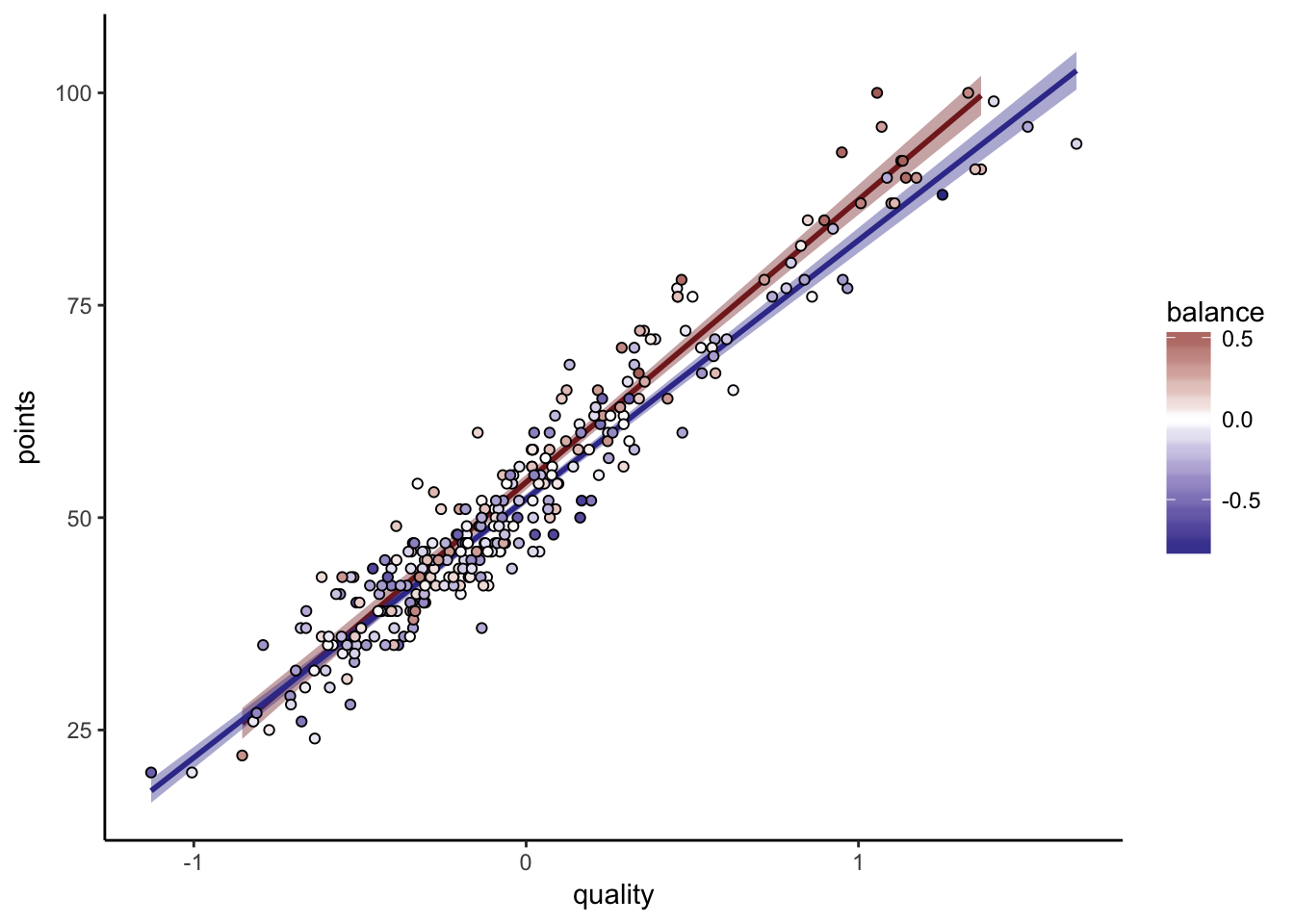
Here the two fits don’t completely separate at the lower end of the scale. Simpson’s paradox and all that. Remember that what we trust the linear fit above better. Fitting one model for attacking teams and another for defensive teams is a very clumsy way to answer the question, but I thought it would at least be easy for people to understand.
The model coefficients are nearly identical to the Premier League ones. I truly, honestly hope there are no “It’s different for La Liga” takes, funny though it would be.
All together
Putting all three leagues together (normalizing Bundesliga points):
##
## Call:
## lm(formula = points ~ quality + quality:balance, data = .)
##
## Residuals:
##      Min       1Q   Median       3Q      Max
## -11.7980  -2.8996  -0.2284   2.4030  11.9613
##
## Coefficients:
##                 Estimate Std. Error t value Pr(>|t|)
## (Intercept)      52.8459     0.2484 212.721  < 2e-16 ***
## quality          32.1389     0.5034  63.844  < 2e-16 ***
## quality:balance   6.6841     1.6117   4.147  4.4e-05 ***
## ---
## Signif. codes:  0 '***' 0.001 '**' 0.01 '*' 0.05 '.' 0.1 ' ' 1
##
## Residual standard error: 4.211 on 297 degrees of freedom
## Multiple R-squared:  0.9321, Adjusted R-squared:  0.9316
## F-statistic:  2038 on 2 and 297 DF,  p-value: < 2.2e-16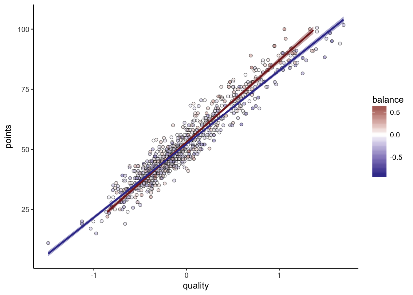
Conclusion
This was interesting, but it should not be necessary. Whether to be offensive or defensive is one of the most basic mathematical questions one can ask about football; it is “Mathematics in Football 101”. It is dispiriting that this should be a matter of confusion. If football analysts can’t even answer this simple question, how could they possibly tackle more complex questions?
Football has little data. Goals are infrequent, and games in different competitions are not immediately comparable. When the data is sparse, it is imperative to use proper mathematical and statistical methodology. Rules of thumb won’t do it, and disregard for the nature of the measurements (i.e. multiplicative count data vs. linearized dimensionless quantities) is disastrous. Humans have spent thousands of years developing mathematics - the least we can do is learn it and use it.